RUEN Research
  • Home
  • Courses
    • Research Methodology
    • Data Analysis Using R
    • Communication and IT
    • Machine Learning Using R
  • Blogs
  • My Courses

Contents

  • Reading data sets

R markdown, Basic functions, Package (tidyverse) installation, Visualization using ggplot()

Author

Professor Dr. Md. Kamrul Hasan

Reading data sets

Before reading a dataset from a folder we need to make sure the dataset is in the working directory. We can set working directory using different methods:

  1. Session > Set Working Directory …..

  2. Typing command

  3. Files tab in the Environment Pane

data = readxl::read_excel('DataSets.xlsx', sheet = 'wrangling', range = 'B7:N507')
head(data)
# A tibble: 6 × 13
    sr.   jan   feb   mar   apr   may   jun   jul   aug   sep   oct   nov   dec
  <dbl> <dbl> <dbl> <dbl> <dbl> <dbl> <dbl> <dbl> <dbl> <dbl> <dbl> <dbl> <dbl>
1     1     0     1     1     0     0     0     0     0     0     0     0     0
2     2     0     1     1     1     0     0     0     0     0     0     0     0
3     3     1     0     1     0     1     0     0     0     0     0     0     0
4     4     0     0     1     1     0     1     0     0     1     0     0     0
5     5     1     0     0     0     0     0     0     0     0     1     0     0
6     6     0     1     0     0     0     0     0     0     0     0     0     0
tail(data)
# A tibble: 6 × 13
    sr.   jan   feb   mar   apr   may   jun   jul   aug   sep   oct   nov   dec
  <dbl> <dbl> <dbl> <dbl> <dbl> <dbl> <dbl> <dbl> <dbl> <dbl> <dbl> <dbl> <dbl>
1   495     0     1     0     1     0     0     1     0     0     0     0     0
2   496     0     1     1     0     0     0     0     0     0     0     0     0
3   497     1     0     1     1     1     0     0     0     0     0     0     0
4   498     0     0     0     1     1     0     1     0     0     0     0     0
5   499     1     0     0     0     0     0     0     0     0     0     0     1
6   500     0     0     0     1     0     0     0     0     0     0     0     0
str(data)
tibble [500 × 13] (S3: tbl_df/tbl/data.frame)
 $ sr.: num [1:500] 1 2 3 4 5 6 7 8 9 10 ...
 $ jan: num [1:500] 0 0 1 0 1 0 0 0 1 0 ...
 $ feb: num [1:500] 1 1 0 0 0 1 1 0 0 0 ...
 $ mar: num [1:500] 1 1 1 1 0 0 0 0 1 1 ...
 $ apr: num [1:500] 0 1 0 1 0 0 1 0 0 1 ...
 $ may: num [1:500] 0 0 1 0 0 0 1 0 1 0 ...
 $ jun: num [1:500] 0 0 0 1 0 0 0 0 1 1 ...
 $ jul: num [1:500] 0 0 0 0 0 0 0 0 0 0 ...
 $ aug: num [1:500] 0 0 0 0 0 0 0 1 0 0 ...
 $ sep: num [1:500] 0 0 0 1 0 0 0 0 0 0 ...
 $ oct: num [1:500] 0 0 0 0 1 0 0 0 0 0 ...
 $ nov: num [1:500] 0 0 0 0 0 0 0 1 0 0 ...
 $ dec: num [1:500] 0 0 0 0 0 0 0 0 0 0 ...
summary(data)
      sr.             jan             feb             mar       
 Min.   :  1.0   Min.   :0.000   Min.   :0.000   Min.   :0.000  
 1st Qu.:125.8   1st Qu.:0.000   1st Qu.:0.000   1st Qu.:0.000  
 Median :250.5   Median :0.000   Median :0.000   Median :0.000  
 Mean   :250.5   Mean   :0.286   Mean   :0.354   Mean   :0.392  
 3rd Qu.:375.2   3rd Qu.:1.000   3rd Qu.:1.000   3rd Qu.:1.000  
 Max.   :500.0   Max.   :1.000   Max.   :1.000   Max.   :1.000  
      apr             may             jun             jul            aug      
 Min.   :0.000   Min.   :0.000   Min.   :0.000   Min.   :0.00   Min.   :0.00  
 1st Qu.:0.000   1st Qu.:0.000   1st Qu.:0.000   1st Qu.:0.00   1st Qu.:0.00  
 Median :0.000   Median :0.000   Median :0.000   Median :0.00   Median :0.00  
 Mean   :0.358   Mean   :0.224   Mean   :0.218   Mean   :0.18   Mean   :0.09  
 3rd Qu.:1.000   3rd Qu.:0.000   3rd Qu.:0.000   3rd Qu.:0.00   3rd Qu.:0.00  
 Max.   :1.000   Max.   :1.000   Max.   :1.000   Max.   :1.00   Max.   :1.00  
      sep             oct            nov             dec       
 Min.   :0.000   Min.   :0.00   Min.   :0.000   Min.   :0.000  
 1st Qu.:0.000   1st Qu.:0.00   1st Qu.:0.000   1st Qu.:0.000  
 Median :0.000   Median :0.00   Median :0.000   Median :0.000  
 Mean   :0.082   Mean   :0.08   Mean   :0.076   Mean   :0.042  
 3rd Qu.:0.000   3rd Qu.:0.00   3rd Qu.:0.000   3rd Qu.:0.000  
 Max.   :1.000   Max.   :1.00   Max.   :1.000   Max.   :1.000  

We will subset the dataset by excluding the Sr. variable (1st variable)
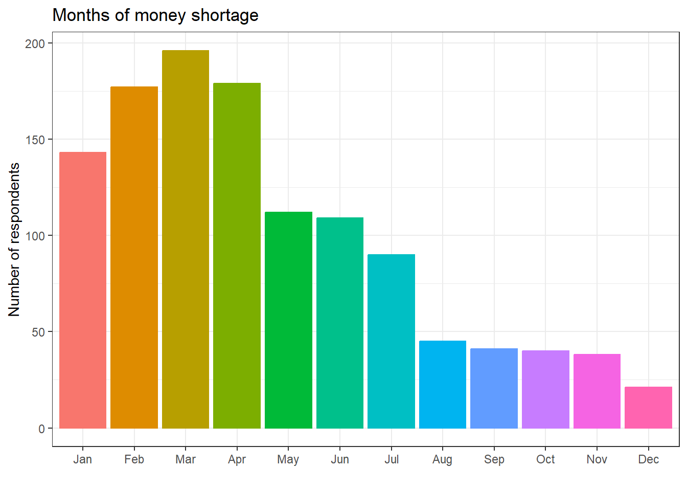
data1 = data[ , -1] 
head(data1)
# A tibble: 6 × 12
    jan   feb   mar   apr   may   jun   jul   aug   sep   oct   nov   dec
  <dbl> <dbl> <dbl> <dbl> <dbl> <dbl> <dbl> <dbl> <dbl> <dbl> <dbl> <dbl>
1     0     1     1     0     0     0     0     0     0     0     0     0
2     0     1     1     1     0     0     0     0     0     0     0     0
3     1     0     1     0     1     0     0     0     0     0     0     0
4     0     0     1     1     0     1     0     0     1     0     0     0
5     1     0     0     0     0     0     0     0     0     1     0     0
6     0     1     0     0     0     0     0     0     0     0     0     0

Calculate the column frequencies (summation) using colSums()

colSums(data1)
jan feb mar apr may jun jul aug sep oct nov dec 
143 177 196 179 112 109  90  45  41  40  38  21 

Create an object to store the value of summation.

sums = as.data.frame(colSums(data1))
str(sums)
'data.frame':   12 obs. of  1 variable:
 $ colSums(data1): num  143 177 196 179 112 109 90 45 41 40 ...
rownames(sums)
 [1] "jan" "feb" "mar" "apr" "may" "jun" "jul" "aug" "sep" "oct" "nov" "dec"

Piping operation: %>% (ctrl+shif+M). It uses the previous output as an input for the next calculation.

library(tidyverse)
Warning: package 'tidyverse' was built under R version 4.5.1
── Attaching core tidyverse packages ──────────────────────── tidyverse 2.0.0 ──
✔ dplyr     1.1.4     ✔ readr     2.1.5
✔ forcats   1.0.0     ✔ stringr   1.5.1
✔ ggplot2   3.5.2     ✔ tibble    3.2.1
✔ lubridate 1.9.4     ✔ tidyr     1.3.1
✔ purrr     1.0.4     
── Conflicts ────────────────────────────────────────── tidyverse_conflicts() ──
✖ dplyr::filter() masks stats::filter()
✖ dplyr::lag()    masks stats::lag()
ℹ Use the conflicted package (<http://conflicted.r-lib.org/>) to force all conflicts to become errors
sums1 = sums %>% rownames_to_column('Months') 
sums1
   Months colSums(data1)
1     jan            143
2     feb            177
3     mar            196
4     apr            179
5     may            112
6     jun            109
7     jul             90
8     aug             45
9     sep             41
10    oct             40
11    nov             38
12    dec             21
sums2 = sums1 %>% rename(Frequency = `colSums(data1)`)
sums2
   Months Frequency
1     jan       143
2     feb       177
3     mar       196
4     apr       179
5     may       112
6     jun       109
7     jul        90
8     aug        45
9     sep        41
10    oct        40
11    nov        38
12    dec        21

Change order of the x-axis items

sums2$Months = factor(sums2$Months, 
                      levels = c('jan', 'feb', 'mar', 'apr', 'may', 'jun', 'jul', 'aug', 'sep', 'oct', 'nov', 'dec' ), 
                      labels = c('Jan', 'Feb', 'Mar', 'Apr', 'May', 'Jun', 'Jul', 'Aug', 'Sep', 'Oct', 'Nov', 'Dec' ))
ggplot(sums2)+
  aes(x = Months, y = Frequency, color = Months, fill = Months)+
  geom_col()+
  theme_bw()+
  labs(title = 'Months of money shortage',
       x = '',
       y = 'Number of respondents')+
  theme(legend.position = '')

ggsave('My plot.png', dpi = 600, height = 4, width = 8, units = 'in')
shortage = as.data.frame(rowSums(data1))
short = shortage %>% rename(frequency = `rowSums(data1)`)
str(short)
'data.frame':   500 obs. of  1 variable:
 $ frequency: num  2 3 3 4 2 1 3 2 4 3 ...
head(short)
  frequency
1         2
2         3
3         3
4         4
5         2
6         1

Some descriptives of this frequency variable.

summary(short)
   frequency    
 Min.   :0.000  
 1st Qu.:1.000  
 Median :2.000  
 Mean   :2.382  
 3rd Qu.:3.000  
 Max.   :9.000  

To see the frequency, we need categorical (factor) variable. Convert the numeric variable to factor variable.

short$frequency = as.factor(short$frequency)
summary(short)
   frequency  
 2      :141  
 3      :113  
 1      :110  
 4      : 69  
 0      : 34  
 5      : 21  
 (Other): 12  
  • Categorize the respondents based on their number of months with money shortage:
  • Two principles: Mutually exclusive, Completely exhaustive
  • Low = up to 3 months of money shortage
  • Medium = 4 to 5 months of money shortage
  • High = >5 months of money shortage
  • For categorization we need numeric (continuous or discrete) variables.
  • Right = TRUE, means right value closed, right value is included in the category
short$frequency = as.numeric(short$frequency)
category = cut(short$frequency, breaks = c(-Inf, 3, 5, Inf), 
    labels = c('Low', 'Medium', 'High'),
    right = TRUE)
table(category)
category
   Low Medium   High 
   285    182     33 

calculate the percentage

table(category)*100/500
category
   Low Medium   High 
  57.0   36.4    6.6 
  • © RUEN Research. All rights reserved.
  • CC BY-NC-SA 4.0
  • Privacy Policy
  • Contact